Distributions

This notebook is an exercise in the Data Visualization course. You can reference the tutorial at this link.

---

In this exercise, you will use your new knowledge to propose a solution to a real-world scenario. To succeed, you will need to import data into Python, answer questions using the data, and generate histograms and density plots to understand patterns in the data.

Scenario

You’ll work with a real-world dataset containing information collected from microscopic images of breast cancer tumors, similar to the image below.

Each tumor has been labeled as either benign (noncancerous) or malignant (cancerous).

To learn more about how this kind of data is used to create intelligent algorithms to classify tumors in medical settings, watch the short video at this link!

Setup

Run the next cell to import and configure the Python libraries that you need to complete the exercise.

import pandas as pd
pd.plotting.register_matplotlib_converters()
import matplotlib.pyplot as plt
%matplotlib inline
import seaborn as sns
print("Setup Complete")

Setup Complete

The questions below will give you feedback on your work. Run the following cell to set up our feedback system.

# Set up code checking
import os
if not os.path.exists("../input/cancer_b.csv"):
    os.symlink("../input/data-for-datavis/cancer_b.csv", "../input/cancer_b.csv")
    os.symlink("../input/data-for-datavis/cancer_m.csv", "../input/cancer_m.csv")
from learntools.core import binder
binder.bind(globals())
from learntools.data_viz_to_coder.ex5 import *
print("Setup Complete")

Setup Complete

Step 1: Load the data

In this step, you will load two data files.

• Load the data file corresponding to benign tumors into a DataFrame called cancer_b_data. The corresponding filepath is cancer_b_filepath. Use the "Id" column to label the rows.
• Load the data file corresponding to malignant tumors into a DataFrame called cancer_m_data. The corresponding filepath is cancer_m_filepath. Use the "Id" column to label the rows.

# Paths of the files to read
cancer_b_filepath = "../input/cancer_b.csv"
cancer_m_filepath = "../input/cancer_m.csv"

# Fill in the line below to read the (benign) file into a variable cancer_b_data
cancer_b_data = pd.read_csv(cancer_b_filepath, index_col="Id")

# Fill in the line below to read the (malignant) file into a variable cancer_m_data
cancer_m_data = pd.read_csv(cancer_m_filepath, index_col="Id")

# Run the line below with no changes to check that you've loaded the data correctly
step_1.check()

<IPython.core.display.Javascript object>

Correct

# Lines below will give you a hint or solution code
#step_1.hint()
#step_1.solution()

Step 2: Review the data

Use a Python command to print the first 5 rows of the data for benign tumors.

# Print the first five rows of the (benign) data
cancer_b_data.head()

	Diagnosis	Radius (mean)	Texture (mean)	Perimeter (mean)	Area (mean)	Smoothness (mean)	Compactness (mean)	Concavity (mean)	Concave points (mean)	Symmetry (mean)	...	Radius (worst)	Texture (worst)	Perimeter (worst)	Area (worst)	Smoothness (worst)	Compactness (worst)	Concavity (worst)	Concave points (worst)	Symmetry (worst)	Fractal dimension (worst)
Id
8510426	B	13.540	14.36	87.46	566.3	0.09779	0.08129	0.06664	0.047810	0.1885	...	15.110	19.26	99.70	711.2	0.14400	0.17730	0.23900	0.12880	0.2977	0.07259
8510653	B	13.080	15.71	85.63	520.0	0.10750	0.12700	0.04568	0.031100	0.1967	...	14.500	20.49	96.09	630.5	0.13120	0.27760	0.18900	0.07283	0.3184	0.08183
8510824	B	9.504	12.44	60.34	273.9	0.10240	0.06492	0.02956	0.020760	0.1815	...	10.230	15.66	65.13	314.9	0.13240	0.11480	0.08867	0.06227	0.2450	0.07773
854941	B	13.030	18.42	82.61	523.8	0.08983	0.03766	0.02562	0.029230	0.1467	...	13.300	22.81	84.46	545.9	0.09701	0.04619	0.04833	0.05013	0.1987	0.06169
85713702	B	8.196	16.84	51.71	201.9	0.08600	0.05943	0.01588	0.005917	0.1769	...	8.964	21.96	57.26	242.2	0.12970	0.13570	0.06880	0.02564	0.3105	0.07409

5 rows × 31 columns

cancer_b_data.info()

<class 'pandas.core.frame.DataFrame'>
Int64Index: 357 entries, 8510426 to 92751
Data columns (total 31 columns):
 #   Column                     Non-Null Count  Dtype  
---  ------                     --------------  -----  
 0   Diagnosis                  357 non-null    object 
 1   Radius (mean)              357 non-null    float64
 2   Texture (mean)             357 non-null    float64
 3   Perimeter (mean)           357 non-null    float64
 4   Area (mean)                357 non-null    float64
 5   Smoothness (mean)          357 non-null    float64
 6   Compactness (mean)         357 non-null    float64
 7   Concavity (mean)           357 non-null    float64
 8   Concave points (mean)      357 non-null    float64
 9   Symmetry (mean)            357 non-null    float64
 10  Fractal dimension (mean)   357 non-null    float64
 11  Radius (se)                357 non-null    float64
 12  Texture (se)               357 non-null    float64
 13  Perimeter (se)             357 non-null    float64
 14  Area (se)                  357 non-null    float64
 15  Smoothness (se)            357 non-null    float64
 16  Compactness (se)           357 non-null    float64
 17  Concavity (se)             357 non-null    float64
 18  Concave points (se)        357 non-null    float64
 19  Symmetry (se)              357 non-null    float64
 20  Fractal dimension (se)     357 non-null    float64
 21  Radius (worst)             357 non-null    float64
 22  Texture (worst)            357 non-null    float64
 23  Perimeter (worst)          357 non-null    float64
 24  Area (worst)               357 non-null    float64
 25  Smoothness (worst)         357 non-null    float64
 26  Compactness (worst)        357 non-null    float64
 27  Concavity (worst)          357 non-null    float64
 28  Concave points (worst)     357 non-null    float64
 29  Symmetry (worst)           357 non-null    float64
 30  Fractal dimension (worst)  357 non-null    float64
dtypes: float64(30), object(1)
memory usage: 89.2+ KB

Use a Python command to print the first 5 rows of the data for malignant tumors.

# Print the first five rows of the (malignant) data
cancer_m_data.head()

	Diagnosis	Radius (mean)	Texture (mean)	Perimeter (mean)	Area (mean)	Smoothness (mean)	Compactness (mean)	Concavity (mean)	Concave points (mean)	Symmetry (mean)	...	Radius (worst)	Texture (worst)	Perimeter (worst)	Area (worst)	Smoothness (worst)	Compactness (worst)	Concavity (worst)	Concave points (worst)	Symmetry (worst)	Fractal dimension (worst)
Id
842302	M	17.99	10.38	122.80	1001.0	0.11840	0.27760	0.3001	0.14710	0.2419	...	25.38	17.33	184.60	2019.0	0.1622	0.6656	0.7119	0.2654	0.4601	0.11890
842517	M	20.57	17.77	132.90	1326.0	0.08474	0.07864	0.0869	0.07017	0.1812	...	24.99	23.41	158.80	1956.0	0.1238	0.1866	0.2416	0.1860	0.2750	0.08902
84300903	M	19.69	21.25	130.00	1203.0	0.10960	0.15990	0.1974	0.12790	0.2069	...	23.57	25.53	152.50	1709.0	0.1444	0.4245	0.4504	0.2430	0.3613	0.08758
84348301	M	11.42	20.38	77.58	386.1	0.14250	0.28390	0.2414	0.10520	0.2597	...	14.91	26.50	98.87	567.7	0.2098	0.8663	0.6869	0.2575	0.6638	0.17300
84358402	M	20.29	14.34	135.10	1297.0	0.10030	0.13280	0.1980	0.10430	0.1809	...	22.54	16.67	152.20	1575.0	0.1374	0.2050	0.4000	0.1625	0.2364	0.07678

5 rows × 31 columns

cancer_m_data.info()

<class 'pandas.core.frame.DataFrame'>
Int64Index: 212 entries, 842302 to 927241
Data columns (total 31 columns):
 #   Column                     Non-Null Count  Dtype  
---  ------                     --------------  -----  
 0   Diagnosis                  212 non-null    object 
 1   Radius (mean)              212 non-null    float64
 2   Texture (mean)             212 non-null    float64
 3   Perimeter (mean)           212 non-null    float64
 4   Area (mean)                212 non-null    float64
 5   Smoothness (mean)          212 non-null    float64
 6   Compactness (mean)         212 non-null    float64
 7   Concavity (mean)           212 non-null    float64
 8   Concave points (mean)      212 non-null    float64
 9   Symmetry (mean)            212 non-null    float64
 10  Fractal dimension (mean)   212 non-null    float64
 11  Radius (se)                212 non-null    float64
 12  Texture (se)               212 non-null    float64
 13  Perimeter (se)             212 non-null    float64
 14  Area (se)                  212 non-null    float64
 15  Smoothness (se)            212 non-null    float64
 16  Compactness (se)           212 non-null    float64
 17  Concavity (se)             212 non-null    float64
 18  Concave points (se)        212 non-null    float64
 19  Symmetry (se)              212 non-null    float64
 20  Fractal dimension (se)     212 non-null    float64
 21  Radius (worst)             212 non-null    float64
 22  Texture (worst)            212 non-null    float64
 23  Perimeter (worst)          212 non-null    float64
 24  Area (worst)               212 non-null    float64
 25  Smoothness (worst)         212 non-null    float64
 26  Compactness (worst)        212 non-null    float64
 27  Concavity (worst)          212 non-null    float64
 28  Concave points (worst)     212 non-null    float64
 29  Symmetry (worst)           212 non-null    float64
 30  Fractal dimension (worst)  212 non-null    float64
dtypes: float64(30), object(1)
memory usage: 53.0+ KB

In the datasets, each row corresponds to a different image. Each dataset has 31 different columns, corresponding to:

• 1 column ('Diagnosis') that classifies tumors as either benign (which appears in the dataset as B) or malignant (M), and
• 30 columns containing different measurements collected from the images.

Use the first 5 rows of the data (for benign and malignant tumors) to answer the questions below.

# Fill in the line below: In the first five rows of the data for benign tumors, what is the
# largest value for 'Perimeter (mean)'?
max_perim = 87.46

# Fill in the line below: What is the value for 'Radius (mean)' for the tumor with Id 842517?
mean_radius = 20.57

# Check your answers
step_2.check()

<IPython.core.display.Javascript object>

Correct

# Lines below will give you a hint or solution code
#step_2.hint()
#step_2.solution()

Step 3: Investigating differences

Part A

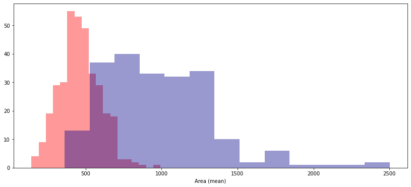
Use the code cell below to create two histograms that show the distribution in values for 'Area (mean)' for both benign and malignant tumors. (To permit easy comparison, create a single figure containing both histograms in the code cell below.)

# Histograms for benign and maligant tumors
plt.figure(figsize=(14,6))
sns.distplot(a=cancer_b_data['Area (mean)'], kde=False, color="red") # Your code here (benign tumors)
sns.distplot(a=cancer_m_data['Area (mean)'], kde=False, color="darkblue") # Your code here (malignant tumors)


# Check your answer
step_3.a.check()

<IPython.core.display.Javascript object>

Correct

# Lines below will give you a hint or solution code
#step_3.a.hint()
#step_3.a.solution_plot()

Part B

A researcher approaches you for help with identifying how the 'Area (mean)' column can be used to understand the difference between benign and malignant tumors. Based on the histograms above,

• Do malignant tumors have higher or lower values for 'Area (mean)' (relative to benign tumors), on average?
• Which tumor type seems to have a larger range of potential values?

#step_3.b.hint()

# Check your answer (Run this code cell to receive credit!)
step_3.b.solution()

<IPython.core.display.Javascript object>

Solution: Malignant tumors have higher values for 'Area (mean)', on average. Malignant tumors have a larger range of potential values.

Step 4: A very useful column

Part A

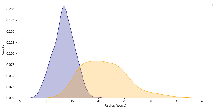
Use the code cell below to create two KDE plots that show the distribution in values for 'Radius (worst)' for both benign and malignant tumors. (To permit easy comparison, create a single figure containing both KDE plots in the code cell below.)

# KDE plots for benign and malignant tumors
plt.figure(figsize=(12, 6))
sns.kdeplot(data=cancer_b_data['Radius (worst)'], shade=True, color="darkblue") # Your code here (benign tumors)
sns.kdeplot(data=cancer_m_data['Radius (worst)'], shade=True, color="orange") # Your code here (malignant tumors)

# Check your answer
step_4.a.check()

plt.legend()

<IPython.core.display.Javascript object>

Correct

<matplotlib.legend.Legend at 0x7f352cb28e90>

# Lines below will give you a hint or solution code
#step_4.a.hint()
#step_4.a.solution_plot()

Part B

A hospital has recently started using an algorithm that can diagnose tumors with high accuracy. Given a tumor with a value for 'Radius (worst)' of 25, do you think the algorithm is more likely to classify the tumor as benign or malignant?

#step_4.b.hint()

# Check your answer (Run this code cell to receive credit!)
step_4.b.solution()

<IPython.core.display.Javascript object>

Solution: The algorithm is more likely to classify the tumor as malignant. This is because the curve for malignant tumors is much higher than the curve for benign tumors around a value of 25 – and an algorithm that gets high accuracy is likely to make decisions based on this pattern in the data.

Keep going

Review all that you’ve learned and explore how to further customize your plots in the next tutorial!

---

Have questions or comments? Visit the course discussion forum to chat with other learners.