Mutual Information

This notebook is an exercise in the Feature Engineering course. You can reference the tutorial at this link.

---

Introduction

In this exercise you’ll identify an initial set of features in the Ames dataset to develop using mutual information scores and interaction plots.

Run this cell to set everything up!

# Setup feedback system
from learntools.core import binder
binder.bind(globals())
from learntools.feature_engineering_new.ex2 import *

import matplotlib.pyplot as plt
import numpy as np
import pandas as pd
import seaborn as sns
from sklearn.feature_selection import mutual_info_regression

# Set Matplotlib defaults
plt.style.use("seaborn-whitegrid")
plt.rc("figure", autolayout=True)
plt.rc(
    "axes",
    labelweight="bold",
    labelsize="large",
    titleweight="bold",
    titlesize=14,
    titlepad=10,
)


# Load data
df = pd.read_csv("../input/fe-course-data/ames.csv")


# Utility functions from Tutorial
def make_mi_scores(X, y):
    X = X.copy()
    for colname in X.select_dtypes(["object", "category"]):
        X[colname], _ = X[colname].factorize()
    # All discrete features should now have integer dtypes
    discrete_features = [pd.api.types.is_integer_dtype(t) for t in X.dtypes]
    mi_scores = mutual_info_regression(X, y, discrete_features=discrete_features, random_state=0)
    mi_scores = pd.Series(mi_scores, name="MI Scores", index=X.columns)
    mi_scores = mi_scores.sort_values(ascending=False)
    return mi_scores


def plot_mi_scores(scores):
    scores = scores.sort_values(ascending=True)
    width = np.arange(len(scores))
    ticks = list(scores.index)
    plt.barh(width, scores)
    plt.yticks(width, ticks)
    plt.title("Mutual Information Scores")

---

To start, let’s review the meaning of mutual information by looking at a few features from the Ames dataset.

features = ["YearBuilt", "MoSold", "ScreenPorch"]
sns.relplot(
    x="value", y="SalePrice", col="variable", data=df.melt(id_vars="SalePrice", value_vars=features), facet_kws=dict(sharex=False),
);

1) Understand Mutual Information

Based on the plots, which feature do you think would have the highest mutual information with SalePrice?

# View the solution (Run this cell to receive credit!)
q_1.check()

<IPython.core.display.Javascript object>

Correct:

Based on the plots, YearBuilt should have the highest MI score since knowing the year tends to constrain SalePrice to a smaller range of possible values. This is generally not the case for MoSold, however. Finally, since ScreenPorch is usually just one value, 0, on average it won’t tell you much about SalePrice (though more than MoSold) .

---

The Ames dataset has seventy-eight features – a lot to work with all at once! Fortunately, you can identify the features with the most potential.

Use the make_mi_scores function (introduced in the tutorial) to compute mutual information scores for the Ames features:

X = df.copy()
y = X.pop('SalePrice')

mi_scores = make_mi_scores(X, y)

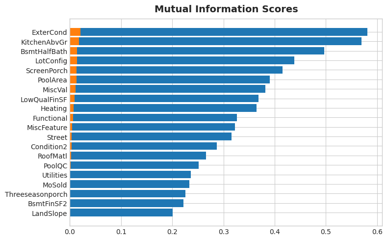
Now examine the scores using the functions in this cell. Look especially at top and bottom ranks.

print(mi_scores.head(20))
print(mi_scores.tail(20))  # uncomment to see bottom 20

plt.figure(dpi=100, figsize=(8, 5))
plot_mi_scores(mi_scores.head(20))
plot_mi_scores(mi_scores.tail(20))  # uncomment to see bottom 20

OverallQual     0.581262
Neighborhood    0.569813
GrLivArea       0.496909
YearBuilt       0.437939
GarageArea      0.415014
TotalBsmtSF     0.390280
GarageCars      0.381467
FirstFlrSF      0.368825
BsmtQual        0.364779
KitchenQual     0.326194
ExterQual       0.322390
YearRemodAdd    0.315402
MSSubClass      0.287131
GarageFinish    0.265440
FullBath        0.251693
Foundation      0.236115
LotFrontage     0.233334
GarageType      0.226117
FireplaceQu     0.221955
SecondFlrSF     0.200658
Name: MI Scores, dtype: float64
ExterCond           0.020934
KitchenAbvGr        0.017677
BsmtHalfBath        0.013719
LotConfig           0.013637
ScreenPorch         0.012981
PoolArea            0.012831
MiscVal             0.010997
LowQualFinSF        0.009328
Heating             0.007622
Functional          0.006380
MiscFeature         0.004322
Street              0.003381
Condition2          0.003176
RoofMatl            0.002620
PoolQC              0.001370
Utilities           0.000291
Threeseasonporch    0.000000
BsmtFinSF2          0.000000
MoSold              0.000000
LandSlope           0.000000
Name: MI Scores, dtype: float64

2) Examine MI Scores

Do the scores seem reasonable? Do the high scoring features represent things you’d think most people would value in a home? Do you notice any themes in what they describe?

# View the solution (Run this cell to receive credit!)
q_2.check()

<IPython.core.display.Javascript object>

Correct:

Some common themes among most of these features are:

• Location: Neighborhood
• Size: all of the Area and SF features, and counts like FullBath and GarageCars
• Quality: all of the Qual features
• Year: YearBuilt and YearRemodAdd
• Types: descriptions of features and styles like Foundation and GarageType

These are all the kinds of features you’ll commonly see in real-estate listings (like on Zillow), It’s good then that our mutual information metric scored them highly. On the other hand, the lowest ranked features seem to mostly represent things that are rare or exceptional in some way, and so wouldn’t be relevant to the average home buyer.

---

In this step you’ll investigate possible interaction effects for the BldgType feature. This feature describes the broad structure of the dwelling in five categories:

Bldg Type (Nominal): Type of dwelling

  1Fam	Single-family Detached	
  2FmCon	Two-family Conversion; originally built as one-family dwelling
  Duplx	Duplex
  TwnhsE	Townhouse End Unit
  TwnhsI	Townhouse Inside Unit

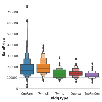
The BldgType feature didn’t get a very high MI score. A plot confirms that the categories in BldgType don’t do a good job of distinguishing values in SalePrice (the distributions look fairly similar, in other words):

sns.catplot(x="BldgType", y="SalePrice", data=df, kind="boxen");

Still, the type of a dwelling seems like it should be important information. Investigate whether BldgType produces a significant interaction with either of the following:

GrLivArea  # Above ground living area
MoSold     # Month sold

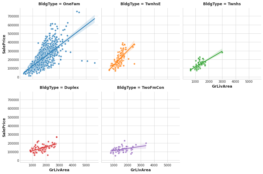
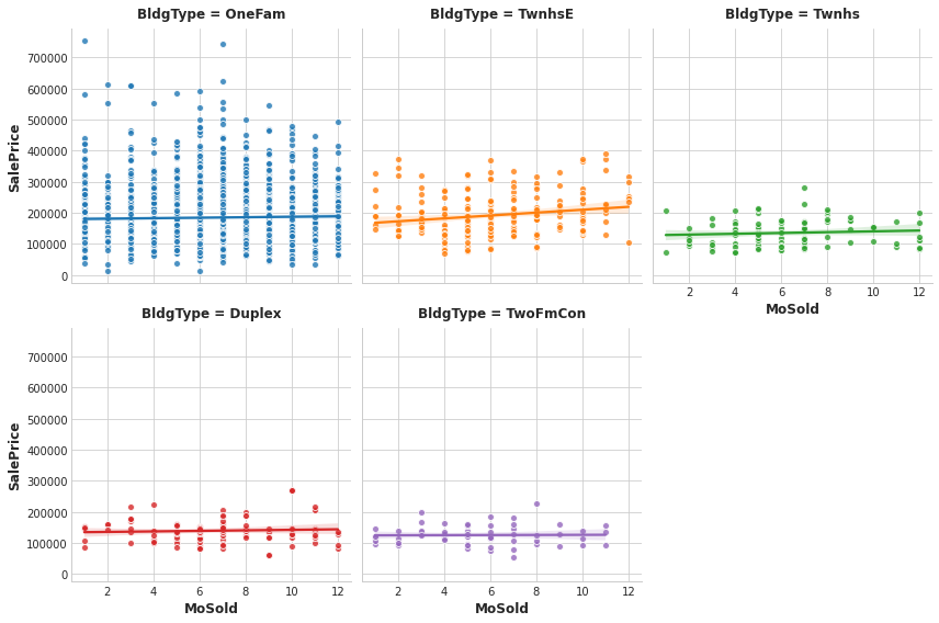
Run the following cell twice, the first time with feature = "GrLivArea" and the next time with feature="MoSold":

# YOUR CODE HERE: 
feature = "GrLivArea"

sns.lmplot(
    x=feature, y="SalePrice", hue="BldgType", col="BldgType",
    data=df, scatter_kws={"edgecolor": 'w'}, col_wrap=3, height=4,
);

feature="MoSold"

sns.lmplot(
    x=feature, y="SalePrice", hue="BldgType", col="BldgType",
    data=df, scatter_kws={"edgecolor": 'w'}, col_wrap=3, height=4,
);

The trend lines being significantly different from one category to the next indicates an interaction effect.

3) Discover Interactions

From the plots, does BldgType seem to exhibit an interaction effect with either GrLivArea or MoSold?

# View the solution (Run this cell to receive credit!)
q_3.check()

<IPython.core.display.Javascript object>

Correct:

The trends lines within each category of BldgType are clearly very different, indicating an interaction between these features. Since knowing BldgType tells us more about how GrLivArea relates to SalePrice, we should consider including BldgType in our feature set.

The trend lines for MoSold, however, are almost all the same. This feature hasn’t become more informative for knowing BldgType.

A First Set of Development Features

Let’s take a moment to make a list of features we might focus on. In the exercise in Lesson 3, you’ll start to build up a more informative feature set through combinations of the original features you identified as having high potential.

You found that the ten features with the highest MI scores were:

mi_scores.head(10)

OverallQual     0.581262
Neighborhood    0.569813
GrLivArea       0.496909
YearBuilt       0.437939
GarageArea      0.415014
TotalBsmtSF     0.390280
GarageCars      0.381467
FirstFlrSF      0.368825
BsmtQual        0.364779
KitchenQual     0.326194
Name: MI Scores, dtype: float64

Do you recognize the themes here? Location, size, and quality. You needn’t restrict development to only these top features, but you do now have a good place to start. Combining these top features with other related features, especially those you’ve identified as creating interactions, is a good strategy for coming up with a highly informative set of features to train your model on.

Keep Going

Start creating features and learn what kinds of transformations different models are most likely to benefit from.

---

Have questions or comments? Visit the course discussion forum to chat with other learners.